Toolbox for the Computation of 2D Fourier Transforms in Polar Coordinates via Maple

Edem Dovlo; Natalie Baddour

(1) Overview

Introduction

Symbolic computation allows a wider range of expression for mathematical formulae and their various transformation rules, while computer algebra admits greater algorithmic precision as it constructs algorithms for computing algebraic quantities in various arithmetic domains. The simplest form of this Fourier transform is the one dimensional case and symbolic computer algebra has successfully been applied to this case.

In Cartesian coordinates, the 2D case is simply two one-dimensional cases (one in each Cartesian direction). However, there are occasions when a system is best expressed in polar coordinates, prompting the need for a Fourier transform in polar coordinates. Recently, the development of the polar coordinate version of a 2D Fourier transform was documented along with the corresponding primary rules [].

In this paper, the development of a Symbolic Computer Algebra (Maple) toolbox for the computation of algebraic, closed-form versions of the two-dimensional Fourier transform in polar coordinates is outlined.

Brief outline of the theory of 2D Fourier transforms in polar coordinates

The 2D Fourier transform of a function f (x, y) is defined as []:

(1)

F (ω →) = F (ω x, ω y) = ∫ − ∞ ∞ ∫ − ∞ ∞ f (x, y) e − j (ω x x + ω y y) d x d y .

M1 \documentclass[10pt]{article} \usepackage{wasysym} \usepackage[substack]{amsmath} \usepackage{amsfonts} \usepackage{amssymb} \usepackage{amsbsy} \usepackage[mathscr]{eucal} \usepackage{mathrsfs} \usepackage{pmc} \usepackage[Euler]{upgreek} \pagestyle{empty} \oddsidemargin -1.0in \begin{document} \[ F\left( {\vec \omega } \right) = F({\omega _x},{\omega _y}) = \int\limits_{ - \infty }^\infty {} \int\limits_{ - \infty }^\infty {f(x,y)} \;{e^{ - j({\omega _x}x + {\omega _y}y)}}dx\;dy. \] \end{document}

The inverse Fourier transform is given by

(2)

f (r →) = f (x, y) = 1 (2 π) 2 ∫ − ∞ ∞ ∫ − ∞ ∞ F (ω x, ω y) e j ω → ⋅ r → d ω x d ω y,

M2 \documentclass[10pt]{article} \usepackage{wasysym} \usepackage[substack]{amsmath} \usepackage{amsfonts} \usepackage{amssymb} \usepackage{amsbsy} \usepackage[mathscr]{eucal} \usepackage{mathrsfs} \usepackage{pmc} \usepackage[Euler]{upgreek} \pagestyle{empty} \oddsidemargin -1.0in \begin{document} \[ f\left( {\vec r} \right) = f(x,y) = \frac{1}{{{{\left( {2\pi } \right)}^2}}}\int\limits_{ - \infty }^\infty {} \int\limits_{ - \infty }^\infty {F({\omega _x},{\omega _y}){e^{j\vec \omega \cdot \vec r}}} d{\omega _x}\;d{\omega _y}, \] \end{document}

where the shorthand notation of $ω → = (ω x, ω y), r → = (x, y)$ M2a \documentclass[10pt]{article} \usepackage{wasysym} \usepackage[substack]{amsmath} \usepackage{amsfonts} \usepackage{amssymb} \usepackage{amsbsy} \usepackage[mathscr]{eucal} \usepackage{mathrsfs} \usepackage{pmc} \usepackage[Euler]{upgreek} \pagestyle{empty} \oddsidemargin -1.0in \begin{document} \[ \vec \omega = ({\omega _x},{\omega _y}),\;\vec r = (x,y) \] \end{document} has been used. Polar coordinates can be introduced as x = r cos θ, y = r sin θ and similarly in the spatial frequency domain as ω_x = ρ cos ψ ω_y = ρ sin ψ otherwise written as, r² = x² + y², θ = arctan (y/x) and ρ² = ω²_x + ω²_y, ψ = arctan (ω_y/ω_x). It then follows that the two-dimensional Fourier transform can be written as

(3)

F (ρ, ψ) = ∫ 0 ∞ ∫ − π π f (r, θ) e − i r ρ cos (ψ − θ) r d r d θ .

M3 \documentclass[10pt]{article} \usepackage{wasysym} \usepackage[substack]{amsmath} \usepackage{amsfonts} \usepackage{amssymb} \usepackage{amsbsy} \usepackage[mathscr]{eucal} \usepackage{mathrsfs} \usepackage{pmc} \usepackage[Euler]{upgreek} \pagestyle{empty} \oddsidemargin -1.0in \begin{document} \[ F\left( {\rho ,\psi } \right) = \int\limits_0^\infty {\int\limits_{ - \pi }^\pi {f(r,\theta )\;{e^{ - ir\rho \cos (\psi - \theta )}}rdr} } d\theta. \] \end{document}

In terms of polar coordinates, the Fourier transform operation transforms the spatial position radius and angle (r, θ) to the frequency radius and angle (ρ, ψ). The corresponding 2D inverse Fourier transform is written as

(4)

f (r, θ) = 1 (2 π) 2 ∫ 0 ∞ ∫ 0 2 π F (ρ, ψ) e j r ρ cos (ψ − θ) d ψ ρ d ρ .

M4 \documentclass[10pt]{article} \usepackage{wasysym} \usepackage[substack]{amsmath} \usepackage{amsfonts} \usepackage{amssymb} \usepackage{amsbsy} \usepackage[mathscr]{eucal} \usepackage{mathrsfs} \usepackage{pmc} \usepackage[Euler]{upgreek} \pagestyle{empty} \oddsidemargin -1.0in \begin{document} \[ f(r,\theta ) = \frac{1}{{{{\left( {2\pi } \right)}^2}}}\int\limits_0^\infty {\int\limits_0^{2\pi } {F(\rho ,\psi ){e^{jr\rho \cos (\psi - \theta )}}} d\psi } \;\rho d\rho. \] \end{document}

A function f (r, θ) expressed in polar coordinates, where r is the radial variable and θ is the angular variable, can be expanded into a Fourier series as

(5)

f (r →) = f (r, θ) = ∑ n = − ∞ ∞ f n (r) e j n θ

M5 \documentclass[10pt]{article} \usepackage{wasysym} \usepackage[substack]{amsmath} \usepackage{amsfonts} \usepackage{amssymb} \usepackage{amsbsy} \usepackage[mathscr]{eucal} \usepackage{mathrsfs} \usepackage{pmc} \usepackage[Euler]{upgreek} \pagestyle{empty} \oddsidemargin -1.0in \begin{document} \[ f\left( {\vec r} \right) = f(r,\theta ) = \sum\limits_{n = - \infty }^\infty {{f_n}(r)\;{e^{jn\theta }}} \] \end{document}

where the Fourier coefficients are given by

(6)

f n (r) = 1 2 π ∫ 0 2 π f (r, θ) e − j n θ d θ .

M6 \documentclass[10pt]{article} \usepackage{wasysym} \usepackage[substack]{amsmath} \usepackage{amsfonts} \usepackage{amssymb} \usepackage{amsbsy} \usepackage[mathscr]{eucal} \usepackage{mathrsfs} \usepackage{pmc} \usepackage[Euler]{upgreek} \pagestyle{empty} \oddsidemargin -1.0in \begin{document} \[ {f_n}(r) = \frac{1}{{2\pi }}\int\limits_0^{2\pi } {f(r,\theta )\;{e^{ - jn\theta }}d\theta }. \] \end{document}

Similarly, the 2D Fourier transform F (ρ, ψ) of f (r, θ) is a function of radial frequency and angular frequency variables (ρ, ψ), and can also be expanded into its own Fourier series so that

(7)

F (ω →) = F (ρ, ψ) = ∑ n = − ∞ ∞ F n (ρ) e j n ψ

M7 \documentclass[10pt]{article} \usepackage{wasysym} \usepackage[substack]{amsmath} \usepackage{amsfonts} \usepackage{amssymb} \usepackage{amsbsy} \usepackage[mathscr]{eucal} \usepackage{mathrsfs} \usepackage{pmc} \usepackage[Euler]{upgreek} \pagestyle{empty} \oddsidemargin -1.0in \begin{document} \[ F\left( {\vec \omega } \right) = F\left( {\rho ,\psi } \right) = \sum\limits_{n = - \infty }^\infty {{F_n}(\rho )\;{e^{jn\psi }}} \] \end{document}

where

(8)

F n (ρ) = 1 2 π ∫ 0 2 π F (ρ, ψ) e − j n ψ d ψ .

M8 \documentclass[10pt]{article} \usepackage{wasysym} \usepackage[substack]{amsmath} \usepackage{amsfonts} \usepackage{amssymb} \usepackage{amsbsy} \usepackage[mathscr]{eucal} \usepackage{mathrsfs} \usepackage{pmc} \usepackage[Euler]{upgreek} \pagestyle{empty} \oddsidemargin -1.0in \begin{document} \[ {F_n}(\rho ) = \frac{1}{{2\pi }}\int\limits_0^{2\pi } {F(\rho ,\psi ){e^{ - jn\psi }}d\psi }. \] \end{document}

It is extremely important to note that F_n(ρ) is NOT the Fourier transform of f_n(r). Complete details of the development are given in [], where it is shown that this relationship is given by

(9)

F n (ρ) = 2 π i − n ∫ 0 ∞ f n (r) J n (ρ r) r d r = 2 π i − n H n {f n (r)}

M9 \documentclass[10pt]{article} \usepackage{wasysym} \usepackage[substack]{amsmath} \usepackage{amsfonts} \usepackage{amssymb} \usepackage{amsbsy} \usepackage[mathscr]{eucal} \usepackage{mathrsfs} \usepackage{pmc} \usepackage[Euler]{upgreek} \pagestyle{empty} \oddsidemargin -1.0in \begin{document} \[ \begin{array}{c} {F_n}\left( \rho \right) = 2\pi \;{i^{ - n}}\int\limits_0^\infty {{f_n}(r){J_n}(\rho r)\;rdr} \\ = 2\pi \;{i^{ - n}}{{\rm{H}}_n}\left\{ {{f_n}(r)} \right\} \end{array} \] \end{document}

where H_n{•} denotes an nth order Hankel transform. The inverse relationship is given by

(10)

f n (r) = i n 2 π ∫ 0 ∞ F n (ρ) J n (ρ r) ρ d ρ = i n 2 π H n {F n (ρ)} .

M10 \documentclass[10pt]{article} \usepackage{wasysym} \usepackage[substack]{amsmath} \usepackage{amsfonts} \usepackage{amssymb} \usepackage{amsbsy} \usepackage[mathscr]{eucal} \usepackage{mathrsfs} \usepackage{pmc} \usepackage[Euler]{upgreek} \pagestyle{empty} \oddsidemargin -1.0in \begin{document} \[ {f_n}(r) = \frac{{{i^n}}}{{2\pi }}\int\limits_0^\infty {{F_n}(\rho ){J_n}(\rho r)\;\rho d\rho } = \frac{{{i^n}}}{{2\pi }}\;{{\rm{H}}_n}\left\{ {{F_n}(\rho )} \right\}. \] \end{document}

Therefore, the nth term in the Fourier series for the original function will Hankel transform into the nth term of the Fourier series of the Fourier transform function. However, it is an nth order Hankel transform for the nth term, so that all the terms are not equivalently transformed.

For reference, the nth order Hankel transform is defined by the integral []

(11)

F ⌢ n (ρ) = H n (f (r)) = ∫ 0 ∞ f (r) J n (ρ r) r d r,

M11 \documentclass[10pt]{article} \usepackage{wasysym} \usepackage[substack]{amsmath} \usepackage{amsfonts} \usepackage{amssymb} \usepackage{amsbsy} \usepackage[mathscr]{eucal} \usepackage{mathrsfs} \usepackage{pmc} \usepackage[Euler]{upgreek} \pagestyle{empty} \oddsidemargin -1.0in \begin{document} \[ {\mathord{\buildrel{\lower3pt\hbox{$\scriptscriptstyle\frown$}} \over F} _n}(\rho ) = {{\rm{H}}_n}\left( {f(r)} \right) = \int\limits_0^\infty {f(r){J_n}(\rho r)rdr}, \] \end{document}

where J_n(z) is the nth order Bessel function with the overhat indicating a Hankel transform as shown in equation (11). Here, n may be an arbitrary real or complex number. The Hankel transform is self-reciprocating and the inversion formula is the same as that given by the forward formula. It is noted that this definition of the Hankel transform is not the same as that used by the built-in Maple function for defining Hankel transforms, therefore another function was written in order to match the definition given in equation (11).

Implementation of 2D Fourier transform in polar coordinates

Most importantly, it can be seen that the operation of finding the 2D Fourier transform F (ρ, ψ) of a function F (r, θ) is equivalent to

First finding its Fourier series coefficients in the angular variable f_n(r), given by equation (6).
Finding the Fourier series coefficient of the Fourier transform, F_n(ρ) via F_n(ρ) = 2π i^-nH_n {f_n(r)}. That is, by finding the nth order Hankel transform (of the spatial radial variable to the spatial frequency radial variable) of the nth coefficient in the Fourier series and appropriately scaling the result.
Finally, taking the inverse Fourier series transform (summing the series) with respect to the frequency angular variable, given by equation (7).

Implementation and architecture

The toolbox created for the evaluation of 2D polar Fourier transforms is called SCAToolbox. It is a symbolic computer algebra toolbox that provides a comprehensive collection of interactive tools suitable for computing mainly the two dimensional Fourier transform of expressions in polar coordinates. SCAToolbox consists of several procedures (this is the term used for “functions” in Maple) and operations as well as tables. One of the packages in SCAToolbox is named the IntegralTrans package. This package contains the procedures, tables and operations necessary for computing some integral transforms.

Set-up of the SCAToolbox

The SCAToolbox is broken into sub packages allowing it to be easy to use and maintain. The code structure is made up of four main sections: 1) creating the toolbox, 2) supporting functions, 3) integral transforms and 4) testing and verification. Creating the toolbox depends on the CAS software being used, in this case Maple.

Supporting functions

Many operations and procedures have been designed and implemented as part of this toolbox. The supporting functions are those operations that do not constitute the core of the toolbox but are vital for the complete and effective functionality of the system. These supporting functions help manage other structures within the toolbox. There are two types of supporting functions within the toolbox.

The first type consists of procedures that perform operations on functions. All the procedures in this group are convolutions (one of the major reasons to implement a Fourier transform). The convolutions implemented include one dimensional and two dimensional convolutions in Cartesian coordinates, angular/circular convolution, radial convolution, two dimensional convolution in polar coordinates and series convolution. As their names suggest, these convolutions convolve different function types and so have different rules that apply to their evaluation. A “Bracket” convolution is implemented to make these convolutions easily accessible and usable – that is, one convolution procedure is defined and the type of convolution desired is passed as an option to the procedure. This makes for less error when trying to evaluate a convolution since the syntax becomes uniform for six different types of convolution. Convolutions can be stand-alone procedures and as such are not placed in the IntegralTrans package of the SCAToolbox. Using these operations therefore does not require loading the IntegralTrans package; downloading and loading the SCAToolbox is sufficient.

Procedures that help manage/manipulate other structures in the toolbox form the other type of supporting functions. These are important to the inner workings of the integral transforms and are stored in the IntegralTrans package within the SCAToolbox. Among these procedures are the takeAlook procedure, addToTable procedure, Ekronecker procedure and EdDirac procedure. The former two procedures help manage the toolbox by manipulating tables.

The takeAlook procedure manipulates tables by comparing the entered function with the list of functions in the first column of the lookup table of interest and returning the mapping result in the second column of the table. A process named pattern matching is used to compare the functions. The entered function has particular properties (arithmetic and variable types, etc.) that are matched to a fitting pattern in the table. With the concept of a lookup table comes the need to add to the table. This is accomplished by implementing the addToTable procedure. This procedure adds an expression and its corresponding transform to a given transform table and makes extending an existing table quite simple.

The Ekronecker procedure provides the Kronecker delta function given the appropriate variables. The need for this operation arose when the built-in kronecker function did not work as expected. In Maple, the integral of a shifted Dirac function is halved at the end points. However, in our theoretical work, the desired result at the endpoints is not halved. The EdDirac procedure therefore redefines the built-in Dirac function so that the result matches the theoretical development.

Integral transforms

The integral transforms implemented in this toolbox include the forward nth order Hankel transform (equation (11)) and its inverse, the forward and inverse one dimensional Fourier series transform (equation (5) and (6)) and the forward and inverse two dimensional Fourier transform in polar coordinates (equations (3) and (4)). When lookup and remember tables fail to return a result, the transforms are evaluated directly by integration. A separate function that calls the direct 2D Fourier transform (which attempts to implement the transform by direct integration, equation (3)) is also included, although we found this approach to be ineffective. If evaluation is unsuccessful, the outputs of the transform procedures are written as they are entered except in the case of the Fourier Series transform and its inverse where the actual integral and sum respectively are returned.

The Hankel transform and 1D Fourier series are implemented by using lookup tables. The 2D Fourier transform in polar coordinates is implemented via the two preceding transforms. Here, it draws on the modular nature of the code to implement the transform. This method is part of the core foundation of this work and involves breaking the 2D polar Fourier transform into three steps.

A summary of the contents of the toolbox is shown in Table 1 where f and g are functions of x, ff and gg are functions of x and y, p and q are functions of r, u and v is a function of ϑ, and pp and qq are functions of r and ϑ. Also, s and w are series in n. Additionally, expr is an arbitrary expression, tablename is the name of the table to consider, procname is the name of the procedure to consider, and ans is the result that maps to expr.

Table 1

Summary of the contents of the toolbox.

Function/Procedure name	Calling Sequence	Description

takeAlook	takeAlook(expr, tablename)	Obtain what maps to expr in tablename
addToTable	addToTable(procname, expr, ans)	Add expr⇔ ans to table associated with procedure, procname
Ekronecker	EKronecker(n, m)	Obtain Kronecker delta function i.e. δ_mn=1, when n=m
EdDirac	EdDirac(a)	Redefines Dirac function so that integral at end points is NOT halved
Conv	Conv(f, g, [x], 1dcartesian)	Bracket Convolution: obtain 1D convolution of f(x) and g(x) in Cartesian coordinates
	Conv(ff, gg, [x, y], 2dcartesian)	obtain 2D convolution of ff(x) and gg(x) in Cartesian coords.
	Conv(pp, qq, [r, ϑ], 2dpolar)	obtain 2D convolution of pp(r, ϑ) and qq(r, ϑ) in polar coords.
	Conv(u, v, [ϑ], angular)	obtain angular convolution of u(ϑ) and v(ϑ)
	Conv(p, q, [r], radial)	obtain radial convolution of p(r) and q(r)
	Conv(s, w, [n], series)	obtain convolution of the infinite series, s(n) and w(n)
OneDCartConv	OneDCartConv(f, g, x)	Obtain 1D convolution of f(x) and g(x) in Cartesian coordinates
TwoDCartConv	TwoDCartConv(ff, gg, x, y)	Obtain 2D convolution of ff(x) and gg(x) in Cartesian coords.
TwoDPolarConv	TwoDPolarConv(pp, qq, r, ϑ)	Obtain 2D convolution of pp(r, ϑ) and qq(r, ϑ) in polar coords.
RadConv	RadConv(p, q, r)	Obtain radial convolution of p(r) and q(r)
AngConv	AngConv(u, v, ϑ)	Obtain angular convolution of u(ϑ) and v(ϑ)
SerConv	SerConv(s, w, n)	Obtain convolution of the infinite series, s(n) and w(n)
Hankel	Hankel(p, r, s, n)	Obtain Hankel transform of p(r) (an expression or list)
InvHankel	InvHankel(P, s, r, n)	Obtain Inverse Hankel transform of P(s) (expression or list)
FS1D	FS1D (f, x, n, range, condition)	Obtain 1D Fourier Series of f(x).
	condition = “coefficientComplex”	Returns complex C_n coefficients
	condition = “coefficientReal”	Returns A₀, A_n, B_n coefficients
	condition = “series”	Returns full sum
InvFS1D	InvFS1D(F, n, x)	Obtain Inverse 1D Fourier Series of F[n]
Polar2DFT	Polar2DFT(pp, r, ϑ, ρ, ψ)	Obtain 2D Polar Fourier transform of pp(r, ϑ) by applying 2πi^-n^*(FS + nth order HT) + iFS
InvPolar2DFT	InvPolar2DFT(PP, ρ, ψ, r, ϑ)	Obtain Inverse 2D Polar Fourier transform of PP(ρ, ψ) by applying (iⁿ/2π)^*(FS + nth order HT) + iFS
DirectPolar2DFT	DirectPolar2DFT(pp, r, ϑ, ρ, ψ)	Evaluate 2D Polar Fourier transform of pp(r, ϑ) from the integral definition
FSH	FSH(pp, r, ϑ, ρ, ψ)	Obtain step-by-step results for 2D Polar Fourier Series-Hankel Transform of pp(r, ϑ) i.e. 2πi^-n^*(FS + nth order HT)
InvFSH	InvFSH(PP, ρ, ψ, r, ϑ)	Obtain step-by-step results for Inverse 2D Polar Fourier Series-Hankel Transform of PP(ρ, ψ) i.e. (iⁿ/2π)^*nth order HT + iFS

Quality control

To ensure that these operations and procedures work well, they have been tested and verified with known examples/data.

Below are examples of some simple functions and their transforms. The results shown in this section involve Maple outputs. ‘MapleIn’ is used to indicate the queries and ‘MapleOut’ gives the output of the toolbox. ‘MapleCommand’ represents executable commands.

Example 1

First to be tested is the 1D convolution in Cartesian coordinates. Theory: A Dirac function convolved (single dimension Cartesian convolution) with any other function returns the function i.e. f (x)^*δ(x) = f (x). This is confirmed via the procedure OneDCartConv.

(12)

MapleIn: O n e D C a r t C o n v (S 2, δ (s), s) MapleOut: s 2

M12 \documentclass[10pt]{article} \usepackage{wasysym} \usepackage[substack]{amsmath} \usepackage{amsfonts} \usepackage{amssymb} \usepackage{amsbsy} \usepackage[mathscr]{eucal} \usepackage{mathrsfs} \usepackage{pmc} \usepackage[Euler]{upgreek} \pagestyle{empty} \oddsidemargin -1.0in \begin{document} \[ \begin{array}{l} {\rm{MapleIn:}}\,\,OneDCartConv({s^2},\delta (s),s)\\ {\rm{MapleOut:}}\,\,{s^2} \end{array} \] \end{document}

The equivalent statement using the “Bracket” version of the convolution is

(13)

MapleIn: C o n v (s 2, δ (s), [s], 1 d c a r t e s i a n) MapleOut: s 2

M13 \documentclass[10pt]{article} \usepackage{wasysym} \usepackage[substack]{amsmath} \usepackage{amsfonts} \usepackage{amssymb} \usepackage{amsbsy} \usepackage[mathscr]{eucal} \usepackage{mathrsfs} \usepackage{pmc} \usepackage[Euler]{upgreek} \pagestyle{empty} \oddsidemargin -1.0in \begin{document} \[ \begin{array}{l} {\rm{MapleIn: }}Conv({s^2},\delta (s),[s],1dcartesian)\\ {\rm{MapleOut: }}{s^2} \end{array} \] \end{document}

It also follows that a shifted Dirac function convolved with any other function gives back the function shifted by the same value i.e. f (x)^*δ(x-x₀) = f (x-x₀). The OneDCartConv procedure also confirms this:

(14)

MapleIn: O n e D C a r t C o n v (1 x, δ (x − 5), x) and/or C o n v (δ (x − 5), 1 x, [x], 1 d c a r t e s i a n) MapleOut: 1 x − 5

M14 \documentclass[10pt]{article} \usepackage{wasysym} \usepackage[substack]{amsmath} \usepackage{amsfonts} \usepackage{amssymb} \usepackage{amsbsy} \usepackage[mathscr]{eucal} \usepackage{mathrsfs} \usepackage{pmc} \usepackage[Euler]{upgreek} \pagestyle{empty} \oddsidemargin -1.0in \begin{document} \[ \begin{array}{c} {\rm{MapleIn: }}OneDCartConv\left( {\frac{1}{x},\delta (x - 5),x} \right){\rm{ and/or}}\\ Conv\left( {\delta (x - 5),\frac{1}{x},[x],1dcartesian} \right)\\ {\rm{MapleOut:}}\frac{1}{{x - 5}} \end{array} \] \end{document}

The above computation shows that the “Bracket” convolution works and that the operation does indeed commute.

Example 2

A list of functions is entered for which the Hankel transform of order 0 of the contents is sought. The output list has the correct order of the transforms within it.

(15)

MapleIn: H a n k e l ([1 r 2 + 22, 1 r 2 + 12], r, s, 0) MapleOut: [e − s 4 s, B e s s e l k (0., s)]

M15 \documentclass[10pt]{article} \usepackage{wasysym} \usepackage[substack]{amsmath} \usepackage{amsfonts} \usepackage{amssymb} \usepackage{amsbsy} \usepackage[mathscr]{eucal} \usepackage{mathrsfs} \usepackage{pmc} \usepackage[Euler]{upgreek} \pagestyle{empty} \oddsidemargin -1.0in \begin{document} \[ \begin{array}{l} {\rm{MapleIn: }}Hankel\left( {\left[ {\frac{1}{{\sqrt {{r^2} + {2^2}} }},\frac{1}{{{r^2} + {1^2}}}} \right],r,s,0} \right)\\ {\rm{MapleOut: }}\left[ {\frac{{{e^{ - s\sqrt 4 }}}}{s},Besselk(0.,s)} \right] \end{array} \] \end{document}

The results of the inverse Hankel transform for the same functions as above are evidence that the Hankel transform is indeed self-reciprocating.

(16)

MapleIn: H a n k e l ([1 s 2 + 22, 1 s 2 + 12], s, r, 0) MapleOut: [e − r 4 r, B e s s e l k (0., r)]

M16 \documentclass[10pt]{article} \usepackage{wasysym} \usepackage[substack]{amsmath} \usepackage{amsfonts} \usepackage{amssymb} \usepackage{amsbsy} \usepackage[mathscr]{eucal} \usepackage{mathrsfs} \usepackage{pmc} \usepackage[Euler]{upgreek} \pagestyle{empty} \oddsidemargin -1.0in \begin{document} \[ \begin{array}{l} {\rm{MapleIn: }}Hankel\left( {\left[ {\frac{1}{{\sqrt {{s^2} + {2^2}} }},\frac{1}{{{s^2} + {1^2}}}} \right],s,r,0} \right)\\ {\rm{MapleOut:}}\left[ {\frac{{{e^{ - r\sqrt 4 }}}}{r},Besselk(0.,r)} \right] \end{array} \] \end{document}

Example 3

The direct form of the 2D polar Fourier transform for the function f =1 is evaluated and tested against the indirect approach using the Hankel and Fourier series transforms.

(17)

MapleIn: D i r e c t P o l a r 2 D F T (1, r, θ, ρ, ψ) MapleOut: ∫ 0 ∞ ∫ 0 2 π r ⋅ e − ρ r cos (ψ − θ) d θ d r

M17 \documentclass[10pt]{article} \usepackage{wasysym} \usepackage[substack]{amsmath} \usepackage{amsfonts} \usepackage{amssymb} \usepackage{amsbsy} \usepackage[mathscr]{eucal} \usepackage{mathrsfs} \usepackage{pmc} \usepackage[Euler]{upgreek} \pagestyle{empty} \oddsidemargin -1.0in \begin{document} \[ \begin{array}{l} {\rm{MapleIn: }}DirectPolar2DFT(1,r,\theta ,\rho ,\psi )\\ {\rm{MapleOut:}}\int_0^\infty {\int_0^{2\pi } {r \cdot {e^{ - \rho r\cos (\psi - \theta )}}} } d\theta dr \end{array} \] \end{document}

The direct method above produces an indeterminate result whereas the indirect method that follows gives a definite and accurate result.

(18)

MapleIn: P o l a r 2 D F T (1, r, θ, ρ, ψ) MapleOut: 2 π δ (ρ) ρ

M18 \documentclass[10pt]{article} \usepackage{wasysym} \usepackage[substack]{amsmath} \usepackage{amsfonts} \usepackage{amssymb} \usepackage{amsbsy} \usepackage[mathscr]{eucal} \usepackage{mathrsfs} \usepackage{pmc} \usepackage[Euler]{upgreek} \pagestyle{empty} \oddsidemargin -1.0in \begin{document} \[ \begin{array}{l} {\rm{MapleIn: }}Polar2DFT(1,r,\theta ,\rho ,\psi )\\ {\rm{MapleOut: }}\frac{{2\pi \delta (\rho )}}{\rho } \end{array} \] \end{document}

A Maple worksheet demonstrating how the toolbox may be used (and including the examples shown above) can be downloaded from http://dx.doi.org/10.6084/m9.figshare.1004937.

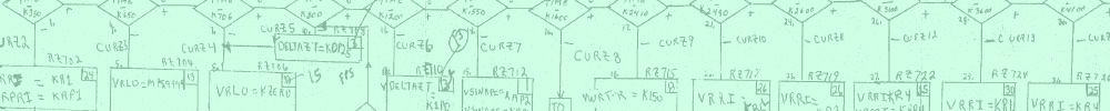
Figure 1 gives a summary of a few functions (including the example above) that were tested and their transforms.

Figure 1

Testing the toolbox on the Fourier transform of some common functions.

(2) Availability

Operating system

Windows XP and higher.

Programming language

Maple version 12 and higher.

Additional system requirements

If using Maple 12, minimum system requirements are 512MB of RAM and 1GB of hard disk space. Higher versions of Maple will required additional memory and disk space.

Dependencies

Maple version 12 and higher

List of contributors

Edem Dovlo and Natalie Baddour

Software location

Name

figshare

Persistent identifier

http://dx.doi.org/10.6084/m9.figshare.1004937

Licence

MIT

Publisher

Natalie Baddour

Date published

23/04/14

The persistent identifier provided above is a link to a complete fileset that includes the toolbox, instructions for downloading and using the toolbox and sample Maple code for using the toolbox.

License

This software is released under the MIT license.

Language

English

Support

Please send email to nbaddour@uottawa.ca or senaedem@gmail.com.

(3) Reuse potential

This software can be used and extended by any researchers who require the use of 2D Fourier Transforms in polar coordinates within a Computer Algebra System environment. The toolbox has only been implemented in the Maple programming language. In particular, the toolbox contains several ‘standalone’ procedures or functions that may be re-used in other code, independently of the toolbox as a whole, in particular all the various forms of convolution that have been implemented.

[B1] Baddour, N. (2009). “Operational and convolution properties of two-dimensional Fourier transforms in polar coordinates,” J. Opt. Soc. Am. A Aug 200926(8): 1767–1777, DOI: https://doi.org/10.1364/JOSAA.26.001767

[B2] Piessens, R. (2000). “The Hankel Transform,” In: The Transforms and Applications Handbook. Second, Boca Raton: CRC Press, pp. 9.1–9.30. http://bit.ly/Qg4VwA

Journal of Open Research Software

Software Metapapers